Black-Scholes Pricing in Python

Let us verify the Black-Scholes call price formula numerically. The closed form is:

$$C = S_0 N(d_1) - K e^{-rT} N(d_2)$$

where the d-terms are $d_1 = \frac{\ln(S_0/K) + (r + \sigma^2/2)T}{\sigma\sqrt{T}}$ and $d_2 = d_1 - \sigma\sqrt{T}$.

import numpy as np
from scipy.stats import norm

def black_scholes_call(S0, K, T, r, sigma):
    d1 = (np.log(S0 / K) + (r + 0.5 * sigma**2) * T) / (sigma * np.sqrt(T))
    d2 = d1 - sigma * np.sqrt(T)
    return S0 * norm.cdf(d1) - K * np.exp(-r * T) * norm.cdf(d2)

black_scholes_call(100, 100, 1, 0.05, 0.2)

np.float64(10.450583572185565)

Visualising the payoff

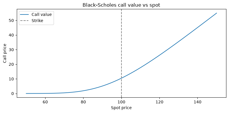
Now let us plot the call option value across a range of spot prices.

import matplotlib.pyplot as plt
S = np.linspace(50, 150, 200)
C = [black_scholes_call(s, 100, 1, 0.05, 0.2) for s in S]
fig, ax = plt.subplots(figsize=(8, 4))
ax.plot(S, C, label='Call value')
ax.axvline(100, color='gray', ls='--', label='Strike')
ax.set_xlabel('Spot price')
ax.set_ylabel('Call price')
ax.legend()
ax.set_title('Black-Scholes call value vs spot')
plt.tight_layout()
plt.show()